# dataset from https://www.kaggle.com/datasets/arthurboari/taylor-swift-spotify-data
#df = pd.read_csv('Taylor Swift Spotify Data 07-23.csv')
# dataset from https://www.kaggle.com/datasets/jarredpriester/taylor-swift-spotify-dataset
import warnings
warnings.simplefilter(action='ignore', category=FutureWarning)

import pandas as pd
import matplotlib.pyplot as plt
import numpy as np
from sklearn.linear_model import LinearRegression
total_records = pd.read_csv('taylor_swift_spotify.csv')

Basic dataframe understanding

Let us get the frameheader to check what is located inside.

total_records.head()

	Unnamed: 0	name	album	release_date	track_number	id	uri	acousticness	danceability	energy	instrumentalness	liveness	loudness	speechiness	tempo	valence	popularity	duration_ms
0	0	Fortnight (feat. Post Malone)	THE TORTURED POETS DEPARTMENT: THE ANTHOLOGY	2024-04-19	1	6dODwocEuGzHAavXqTbwHv	spotify:track:6dODwocEuGzHAavXqTbwHv	0.5020	0.504	0.386	0.000015	0.0961	-10.976	0.0308	192.004	0.281	82	228965
1	1	The Tortured Poets Department	THE TORTURED POETS DEPARTMENT: THE ANTHOLOGY	2024-04-19	2	4PdLaGZubp4lghChqp8erB	spotify:track:4PdLaGZubp4lghChqp8erB	0.0483	0.604	0.428	0.000000	0.1260	-8.441	0.0255	110.259	0.292	79	293048
2	2	My Boy Only Breaks His Favorite Toys	THE TORTURED POETS DEPARTMENT: THE ANTHOLOGY	2024-04-19	3	7uGYWMwRy24dm7RUDDhUlD	spotify:track:7uGYWMwRy24dm7RUDDhUlD	0.1370	0.596	0.563	0.000000	0.3020	-7.362	0.0269	97.073	0.481	80	203801
3	3	Down Bad	THE TORTURED POETS DEPARTMENT: THE ANTHOLOGY	2024-04-19	4	1kbEbBdEgQdQeLXCJh28pJ	spotify:track:1kbEbBdEgQdQeLXCJh28pJ	0.5600	0.541	0.366	0.000001	0.0946	-10.412	0.0748	159.707	0.168	82	261228
4	4	So Long, London	THE TORTURED POETS DEPARTMENT: THE ANTHOLOGY	2024-04-19	5	7wAkQFShJ27V8362MqevQr	spotify:track:7wAkQFShJ27V8362MqevQr	0.7300	0.423	0.533	0.002640	0.0816	-11.388	0.3220	160.218	0.248	80	262974

Let us replace the capital lettered long album with smething small and readable.

total_records = total_records.replace('THE TORTURED POETS DEPARTMENT', 'TTPD', regex=True)
total_records = total_records.replace('THE ANTHOLOGY', 'The anthology', regex=True)

Filter unwanted albums to get the albums only. This involves the Big Machine versions and Taylor’s versions.

# filter the rows that contain the substring, this is to remove entries which aren't original albums but special renditions and such
substring = ['Deluxe','Disney', 'Live','Stadium','delux','International','Piano']
pattern = '|'.join(substring)

filter = total_records['album'].str.contains(pattern) 
filtered_df = total_records[~filter]

print(filtered_df['album'].unique())
filtered_df.groupby(['album']).size().sum()

['TTPD: The anthology' 'TTPD' "1989 (Taylor's Version)"
 "Speak Now (Taylor's Version)" 'Midnights (The Til Dawn Edition)'
 'Midnights (3am Edition)' 'Midnights' "Red (Taylor's Version)"
 "Fearless (Taylor's Version)" 'evermore' 'folklore' 'Lover' 'reputation'
 '1989' 'Red' 'Speak Now' 'Fearless (Platinum Edition)']





328

Album summaries

This will be album summary. This should act as a one stop shop to quickly get an overview of what’s happening for each album.

album_summary=pd.DataFrame()
album_summary['album']=filtered_df.groupby(['album'])['speechiness'].min().keys()
album_summary['size']=list(filtered_df.groupby(['album']).size())
album_summary['speechiness_min']=list(filtered_df.groupby(['album'])['speechiness'].min())
album_summary['speechiness_max']=list(filtered_df.groupby(['album'])['speechiness'].max())
album_summary['loudness_min']=list(filtered_df.groupby(['album'])['loudness'].min())
album_summary['loudness_max']=list(filtered_df.groupby(['album'])['loudness'].max())
album_summary['total_duration_ms']=list(filtered_df.groupby(['album'])['duration_ms'].sum())
album_summary['total_duration_HMS'] = pd.to_datetime(album_summary['total_duration_ms'], unit='ms').dt.strftime('%H:%M:%S:%f').str[:-3] 
album_summary['mean_popularity'] =  list(filtered_df.groupby(['album'])['popularity'].mean())
album_summary

	album	size	speechiness_min	speechiness_max	loudness_min	loudness_max	total_duration_ms	total_duration_HMS	mean_popularity
0	1989	13	0.0324	0.1810	-8.768	-4.807	2927864	00:48:47:864	52.692308
1	1989 (Taylor's Version)	21	0.0303	0.1590	-13.187	-4.803	4678327	01:17:58:327	72.190476
2	Fearless (Platinum Edition)	19	0.0239	0.0549	-10.785	-3.096	4766608	01:19:26:608	43.157895
3	Fearless (Taylor's Version)	26	0.0263	0.0628	-11.548	-3.669	6392490	01:46:32:490	65.269231
4	Lover	18	0.0344	0.5190	-12.566	-4.105	3711381	01:01:51:381	75.944444
5	Midnights	13	0.0349	0.3870	-15.512	-6.645	2648338	00:44:08:338	74.153846
6	Midnights (3am Edition)	20	0.0342	0.3870	-15.512	-6.557	4169264	01:09:29:264	62.850000
7	Midnights (The Til Dawn Edition)	23	0.0342	0.3870	-15.512	-6.548	4835165	01:20:35:165	62.434783
8	Red	16	0.0243	0.0916	-12.411	-4.267	3895394	01:04:55:394	45.000000
9	Red (Taylor's Version)	30	0.0250	0.1750	-13.778	-4.516	7839830	02:10:39:830	67.233333
10	Speak Now	14	0.0258	0.0887	-9.531	-2.641	4021982	01:07:01:982	50.714286
11	Speak Now (Taylor's Version)	22	0.0263	0.0771	-8.641	-1.927	6284051	01:44:44:051	69.454545
12	TTPD	16	0.0255	0.3220	-13.961	-7.123	3915705	01:05:15:705	77.000000
13	TTPD: The anthology	31	0.0255	0.3220	-13.961	-4.514	7358744	02:02:38:744	78.774194
14	evermore	15	0.0264	0.2450	-12.077	-7.589	3645210	01:00:45:210	66.400000
15	folklore	16	0.0253	0.0916	-15.065	-6.942	3816587	01:03:36:587	72.812500
16	reputation	15	0.0354	0.1960	-12.864	-5.986	3345300	00:55:45:300	75.733333

Simple visual representation

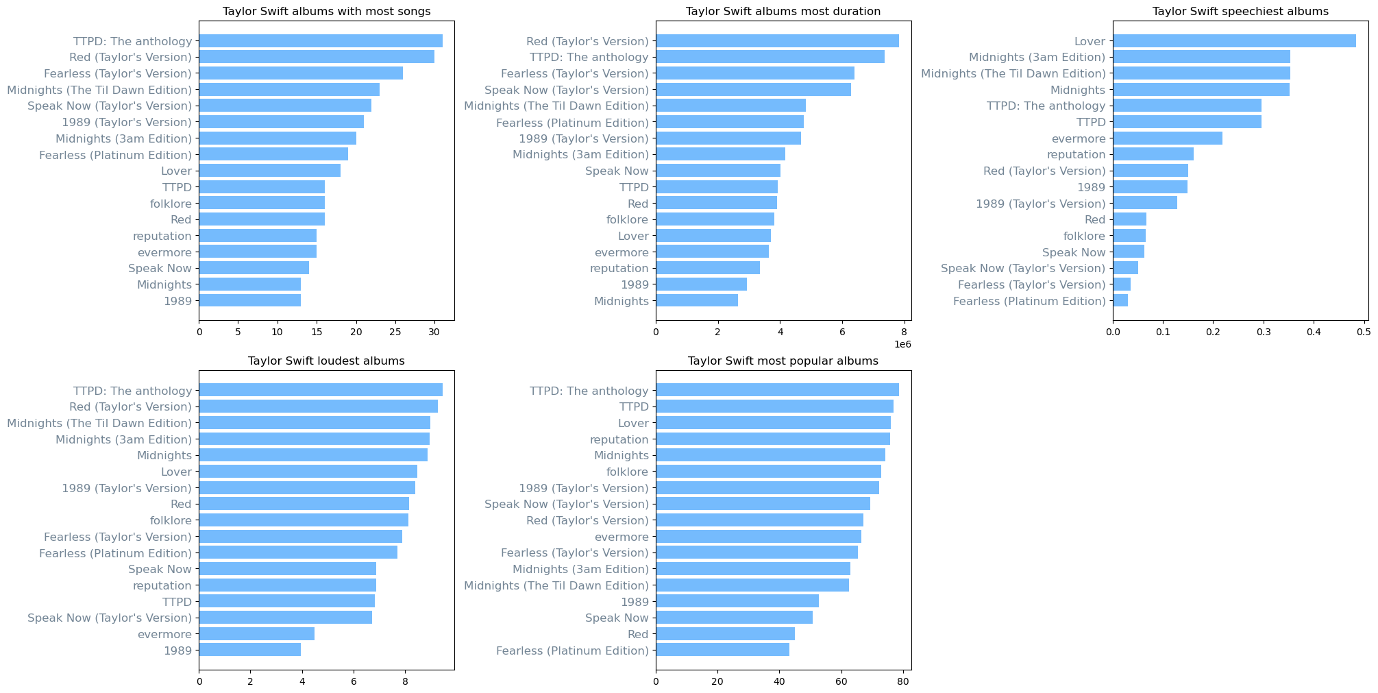
Which of her albums are longest, most popular, or loudest? Here are histograms representing that. For each histogram the corresponding criteria is sorted upon. It is clear that Taylor’s versions are considerably more popular than the Big Machine versions.

fig, ax = plt.subplots(2,3, figsize = (20,10), layout="constrained" )#, sharex=True)#, sharey=True)
fig.delaxes(ax[1][2])
temp_df=pd.DataFrame()
temp_df['album']=album_summary['album'].astype(str)
temp_df['size']=album_summary['size']
temp_df['total_duration_ms']=album_summary['total_duration_ms']
temp_df['speechiness']= abs(album_summary['speechiness_min']-album_summary['speechiness_max'])
temp_df['loudness']= abs(album_summary['loudness_min'])-abs(album_summary['loudness_max'])
temp_df['popularity']= album_summary['mean_popularity']

criteria = ['size', 'total_duration_ms', 'speechiness', 'loudness','popularity']
plot_title = ['Taylor Swift albums with most songs','Taylor Swift albums most duration','Taylor Swift speechiest albums',\
              'Taylor Swift loudest albums', 'Taylor Swift most popular albums']
for i in range(len(criteria)): 
    temp_df = temp_df.sort_values(by=[criteria[i]])
    #print(temp_df['loudness'])
    if i <= 2:
        #ax[0][0]=temp_df.plot.barh(color = 'xkcd:steel')
        ax[0][i].barh(temp_df['album'],temp_df[criteria[i]], color = 'xkcd:sky blue')
        ax[0][i].set_yticks(range(len(list(temp_df['album']))), temp_df['album'], fontsize=12, color = 'xkcd:steel');
        ax[0][i].set_title(plot_title[i]);
    else:
        #ax[0][0]=temp_df.plot.barh(color = 'xkcd:steel')
        ax[1][i-3].barh(temp_df['album'],temp_df[criteria[i]], color = 'xkcd:sky blue')
        ax[1][i-3].set_yticks(range(len(list(temp_df['album']))), temp_df['album'], fontsize=12, color = 'xkcd:steel');
        ax[1][i-3].set_title(plot_title[i]);

Starting to gain some insights

I want to get some insights into these variables without knowing the definitions. This is not a very good idea of course but I want to first know if some of the variables in the dataframe are correlated. If so which ones? Here I also make first contact with scikit-learn and use the LinearRegression model to check for the correlation. What I use here is the $R^2$ which should be the square of the correlation coefficient. I also show the model coefficient which should tell us if the data is correlated or anticorrelated.

import matplotlib.pyplot as plt
import numpy as np

xvals = ['loudness', 'energy', 'speechiness', 'danceability','acousticness','liveness','tempo','valence','popularity','instrumentalness']
yvals = ['loudness', 'energy', 'speechiness', 'danceability','acousticness','liveness','tempo','valence','popularity','instrumentalness']

newxcol = []
newycol = []
for i in range(len(xvals)):
    for j in range(len(yvals)):
        if i >=j: continue
        xcol = filtered_df[xvals[i]]
        ycol = filtered_df[yvals[j]]
        x = np.array(list(xcol)).reshape((-1,1))
        y = np.array(list(ycol))
        model = LinearRegression().fit(x,y)
        rsq = model.score(x, y)
        if rsq > 0.1: 
            print(f"overall coefficient of determination for : {xvals[i], yvals[j], rsq,  model.coef_[0]}")
            newxcol.append(xvals[i])
            newycol.append(yvals[j])

overall coefficient of determination for : ('loudness', 'energy', 0.6429955130707232, 0.05193931977241491)
overall coefficient of determination for : ('loudness', 'acousticness', 0.5417812284681403, -0.08155677230919023)
overall coefficient of determination for : ('loudness', 'valence', 0.14387666725197357, 0.02614074917825036)
overall coefficient of determination for : ('energy', 'acousticness', 0.47234085351213695, -1.1756648168955814)
overall coefficient of determination for : ('energy', 'valence', 0.24517689187957725, 0.5268297925424761)

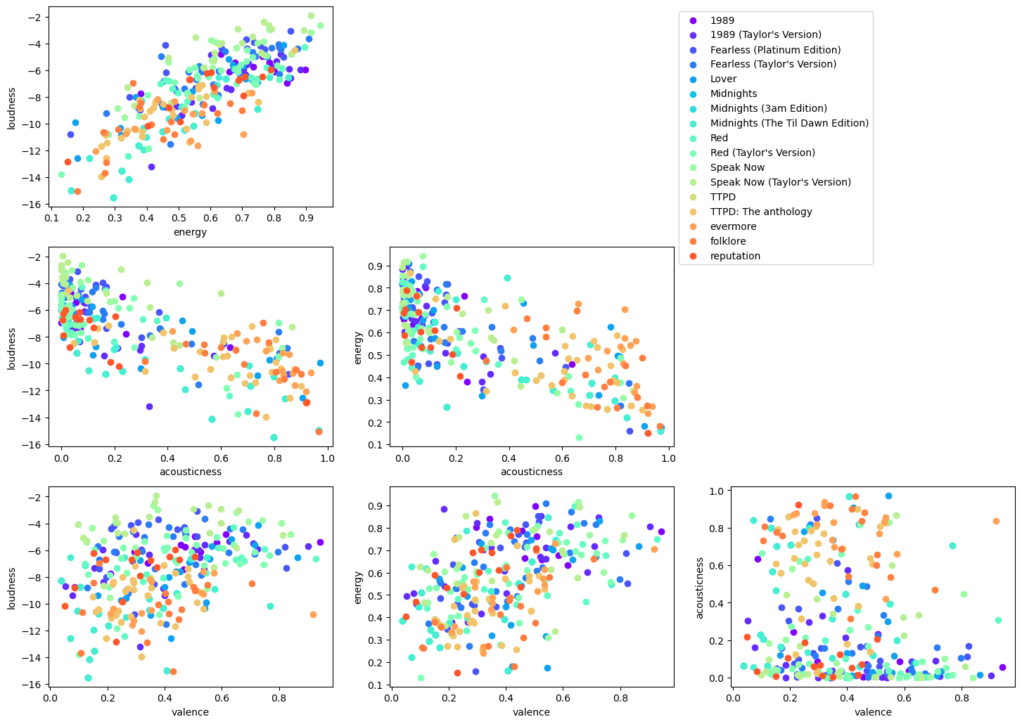
Does the above analysis look good? Let’s inspect visually by plotting the corresponding variables against each other. Note that this part of the code is a bit dirty, I think this can be cleaned up but I will get to it as I go ahead in this project.

The plots below show exactly what we expect from numbers above e.g. energy and loudness are directly correlated to each other but loudness and acousticness are anticorrelated. So it would seem that my understanding of how sklearn linear regression should behave is not too wrong.

# this needs to be iterated over fixed list of colors
import matplotlib.pyplot as plt
import numpy as np
from itertools import cycle
import sys
from matplotlib.pyplot import cm


color = cm.rainbow(np.linspace(0, 1, 19))

xvals = ['loudness', 'energy','acousticness','valence']
yvals = ['loudness', 'energy','acousticness','valence']

fig, ax = plt.subplots(len(xvals), len(yvals), figsize = (24,17), layout="constrained" )#, sharex=True)#, sharey=True)

plot = []
labels = []
for i in range(len(xvals)):
    for j in range(len(yvals)):
        try: 
            if j >= i: fig.delaxes(ax[i][j])
        except: continue
        k = 0
        for x in filtered_df.groupby(['album']).groups:
        #for name, x in filtered_df.groupby(['album']):
            xcol = filtered_df.groupby(['album']).get_group(x)[xvals[i]]
            ycol = filtered_df.groupby(['album']).get_group(x)[yvals[j]]
            album = list(filtered_df.groupby(['album']).get_group(x)['album'])[0]
            #ax[i][j].scatter(xcol, ycol, color=color[k], label = list(name[0]))
            ax[i][j].scatter(xcol, ycol, color=color[k], label = album)
            #ax[i][j].scatter(xcol, ycol, color=next(color), label = list(filtered_df.groupby(['album']).get_group(x)['album'])[0])
            ax[i][j].set_xlabel(xvals[i])
            ax[i][j].set_ylabel(yvals[j])
            if (i == 1 and j == 0): ax[i][j].legend(bbox_to_anchor=(2.2, 1),loc='upper left')#, borderaxespad=0.)
            k = k + 1
fig.subplots_adjust(bottom=0.2)
plt.tight_layout()
plt.show()

/var/folders/zf/vn2shr2j6x9_qkg68dw_nk4c0000gn/T/ipykernel_53361/1207867289.py:36: UserWarning: This figure was using a layout engine that is incompatible with subplots_adjust and/or tight_layout; not calling subplots_adjust.
  fig.subplots_adjust(bottom=0.2)
/var/folders/zf/vn2shr2j6x9_qkg68dw_nk4c0000gn/T/ipykernel_53361/1207867289.py:37: UserWarning: Tight layout not applied. tight_layout cannot make Axes width small enough to accommodate all Axes decorations
  plt.tight_layout()
/var/folders/zf/vn2shr2j6x9_qkg68dw_nk4c0000gn/T/ipykernel_53361/1207867289.py:37: UserWarning: The figure layout has changed to tight
  plt.tight_layout()

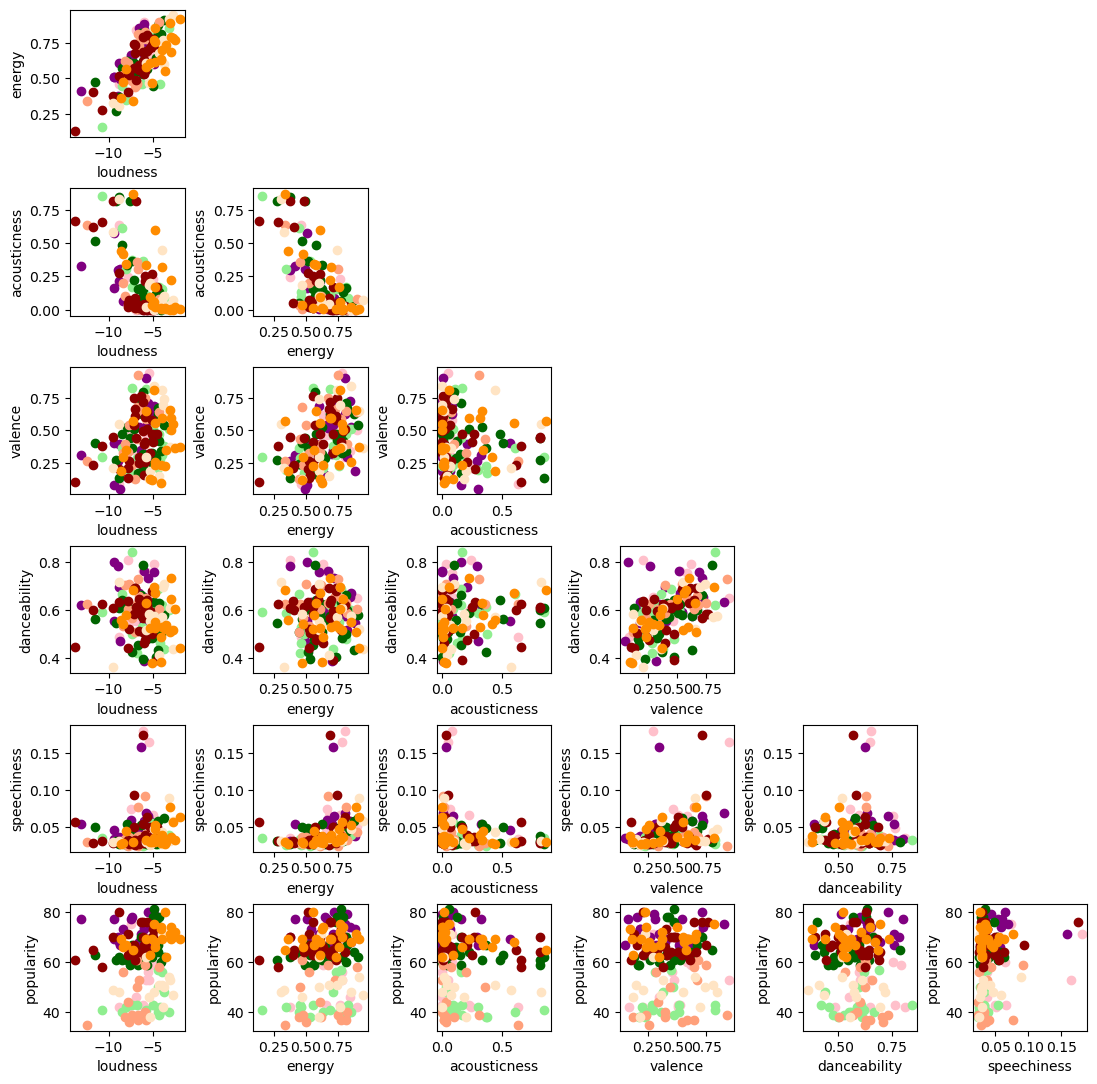
Big Machine versions against Taylor’s versions

What are the differences in Taylor’s versions and the Big Machines versions? I want to answer this question. I didn’t get to it completely because of two reasons: 1) The data was actually a bit faulty in that some of the entries have the wrong encoding for apostrophy. I checked it using ‘cat -v’ command. It was easy to go into the text file and clean it up, but I would like to have an automated way to clean it up. I didn’t find it yet. 2) I still haven’t found a way to filter on the same songs between Big Machine and Taylor’s versions. It would be foolish to compare entire albums here because Taylor’s versions includes considerably more songs.

What I can definitely say is that there is no obvious difference between Taylor’s versions and Big Machine’s versions. This is something you know of course if you are a Swifty. I think this is where her fanbase loyalty really shines.

xvals = ['loudness', 'energy','acousticness','valence','danceability','speechiness','popularity']
yvals = ['loudness', 'energy','acousticness','valence','danceability','speechiness','popularity']
color_BM = ['pink','lightgreen','lightsalmon','bisque']
color_Taylor = ['purple','darkgreen','darkred','darkorange']

temp_df=pd.DataFrame()

substring = ['1989', 'Fearless', 'Red', 'Speak Now']
pattern = '|'.join(substring)

filter = filtered_df['album'].str.contains(pattern)
temp_df = filtered_df[filter]

filter = temp_df['album'].str.contains('Version')

BM_version_temp = temp_df[~filter]
BM_version = BM_version_temp.replace('Fearless \(Platinum Edition\)', 'Fearless', regex=True)

Taylor_version = temp_df[filter]

fig, ax = plt.subplots(len(xvals),len(yvals), figsize = (12,12), layout="constrained" )
for i in range(len(xvals)):
    for j in range(len(yvals)):
      try: 
        if j >= i: fig.delaxes(ax[i][j])
      except: continue
      k = 0
      for BM_name, BM_group in BM_version.groupby(['album']):
        xcol = list(BM_group[xvals[i]])
        ycol = list(BM_group[yvals[j]])
        ax[i][j].scatter(ycol, xcol, color=color_BM[k])
        for Taylor_name, Taylor_group in Taylor_version.groupby(['album']):
            if list(BM_name)[0] in list(Taylor_name)[0]: 
                xcol = list(Taylor_group[xvals[i]])
                ycol = list(Taylor_group[yvals[j]])
                ax[i][j].scatter(ycol, xcol, color=color_Taylor[k])
                ax[i][j].set_xlabel(xvals[j])
                ax[i][j].set_ylabel(yvals[i])
        k = k + 1

Getting to statistics 101

Let’s try to extract some statistics from her data. I plot here the correlation coefficient between the numerical data. I find two surprises 1) I don’t understand why track_number should be related to acusticness. A simple plot didn’t show any such correlation. This needs investigation. 2) Some of the correlation coefficients don’t match with the scikit-learn linear regression analysis, even if I account for the $R^2$ vs $R$ definitions. Perhaps the two are done differently, I need to find this out.

f = plt.figure(figsize=(6, 6))
Taylor_numbers = Taylor_version.drop(['album', 'name','release_date','id','uri','Unnamed: 0'], axis=1)
corr=Taylor_numbers.corr()
corr.style.background_gradient(cmap='coolwarm').format("{:.2f}")

	track_number	acousticness	danceability	energy	instrumentalness	liveness	loudness	speechiness	tempo	valence	popularity	duration_ms
track_number	1.00	0.40	-0.00	-0.26	-0.15	-0.22	-0.40	-0.04	-0.08	-0.08	-0.31	0.13
acousticness	0.40	1.00	0.11	-0.69	-0.09	-0.02	-0.60	-0.19	-0.09	-0.15	-0.32	0.15
danceability	-0.00	0.11	1.00	-0.01	-0.07	-0.18	-0.17	-0.02	-0.36	0.44	0.14	-0.25
energy	-0.26	-0.69	-0.01	1.00	0.13	0.12	0.74	0.31	0.04	0.45	0.27	-0.32
instrumentalness	-0.15	-0.09	-0.07	0.13	1.00	-0.05	0.06	0.02	-0.08	-0.07	0.19	-0.04
liveness	-0.22	-0.02	-0.18	0.12	-0.05	1.00	0.22	-0.03	0.07	-0.09	-0.06	0.00
loudness	-0.40	-0.60	-0.17	0.74	0.06	0.22	1.00	0.06	0.07	0.28	0.20	-0.04
speechiness	-0.04	-0.19	-0.02	0.31	0.02	-0.03	0.06	1.00	0.32	0.30	0.17	-0.26
tempo	-0.08	-0.09	-0.36	0.04	-0.08	0.07	0.07	0.32	1.00	0.05	-0.14	-0.02
valence	-0.08	-0.15	0.44	0.45	-0.07	-0.09	0.28	0.30	0.05	1.00	0.13	-0.38
popularity	-0.31	-0.32	0.14	0.27	0.19	-0.06	0.20	0.17	-0.14	0.13	1.00	0.06
duration_ms	0.13	0.15	-0.25	-0.32	-0.04	0.00	-0.04	-0.26	-0.02	-0.38	0.06	1.00

<Figure size 600x600 with 0 Axes>

xvals = ['loudness', 'energy', 'speechiness', 'danceability','acousticness','liveness','tempo','valence','popularity','instrumentalness','track_number']
yvals = ['loudness', 'energy', 'speechiness', 'danceability','acousticness','liveness','tempo','valence','popularity','instrumentalness','track_number']
newxcol = []
newycol = []
for i in range(len(xvals)):
    for j in range(len(yvals)):
        if i >=j: continue
        xcol = filtered_df[xvals[i]]
        ycol = filtered_df[yvals[j]]
        x = np.array(list(xcol)).reshape((-1,1))
        y = np.array(list(ycol))
        model = LinearRegression().fit(x,y)
        rsq = model.score(x, y)
        if rsq > 0.1: 
            print(f"overall coefficient of determination for : {xvals[i], yvals[j], np.sqrt(rsq),  model.coef_[0]}")
            newxcol.append(xvals[i])
            newycol.append(yvals[j])

overall coefficient of determination for : ('loudness', 'energy', 0.8018700100831326, 0.05193931977241491)
overall coefficient of determination for : ('loudness', 'acousticness', 0.7360578974972962, -0.08155677230919023)
overall coefficient of determination for : ('loudness', 'valence', 0.3793107792456913, 0.02614074917825036)
overall coefficient of determination for : ('energy', 'acousticness', 0.6872705824579842, -1.1756648168955814)
overall coefficient of determination for : ('energy', 'valence', 0.4951534023709998, 0.5268297925424761)