
Suchita Kulkarni, PhD
Suchita Kulkarni, PhD
Photo of Dr. Kulkarni
import pandas as pd
import seaborn as sns
import matplotlib.pyplot as plt
from ipywidgets import *
%matplotlib inline
EDA
Let us make some elementary charts and plots to understand what the data is like.
df_PCOS_all = pd.read_excel('PCOS_data_without_infertility.xlsx', sheet_name = 'Full_new')
df_PCOS_all.head()
| Sl. No | Patient File No. | PCOS (Y/N) | Age (yrs) | Weight (Kg) | Height(Cm) | BMI | Blood Group | Pulse rate(bpm) | RR (breaths/min) | ... | Fast food (Y/N) | Reg.Exercise(Y/N) | BP _Systolic (mmHg) | BP _Diastolic (mmHg) | Follicle No. (L) | Follicle No. (R) | Avg. F size (L) (mm) | Avg. F size (R) (mm) | Endometrium (mm) | Unnamed: 44 | |
|---|---|---|---|---|---|---|---|---|---|---|---|---|---|---|---|---|---|---|---|---|---|
| 0 | 1 | 1 | 0 | 28 | 44.6 | 152.0 | 19.300000 | 15 | 78 | 22 | ... | 1.0 | 0 | 110 | 80 | 3 | 3 | 18.0 | 18.0 | 8.5 | NaN |
| 1 | 2 | 2 | 0 | 36 | 65.0 | 161.5 | 24.921163 | 15 | 74 | 20 | ... | 0.0 | 0 | 120 | 70 | 3 | 5 | 15.0 | 14.0 | 3.7 | NaN |
| 2 | 3 | 3 | 1 | 33 | 68.8 | 165.0 | 25.270891 | 11 | 72 | 18 | ... | 1.0 | 0 | 120 | 80 | 13 | 15 | 18.0 | 20.0 | 10.0 | NaN |
| 3 | 4 | 4 | 0 | 37 | 65.0 | 148.0 | 29.674945 | 13 | 72 | 20 | ... | 0.0 | 0 | 120 | 70 | 2 | 2 | 15.0 | 14.0 | 7.5 | NaN |
| 4 | 5 | 5 | 0 | 25 | 52.0 | 161.0 | 20.060954 | 11 | 72 | 18 | ... | 0.0 | 0 | 120 | 80 | 3 | 4 | 16.0 | 14.0 | 7.0 | NaN |
5 rows × 45 columns
df_PCOS_all.describe()
| Sl. No | Patient File No. | PCOS (Y/N) | Age (yrs) | Weight (Kg) | Height(Cm) | BMI | Blood Group | Pulse rate(bpm) | RR (breaths/min) | ... | Pimples(Y/N) | Fast food (Y/N) | Reg.Exercise(Y/N) | BP _Systolic (mmHg) | BP _Diastolic (mmHg) | Follicle No. (L) | Follicle No. (R) | Avg. F size (L) (mm) | Avg. F size (R) (mm) | Endometrium (mm) | |
|---|---|---|---|---|---|---|---|---|---|---|---|---|---|---|---|---|---|---|---|---|---|
| count | 541.000000 | 541.000000 | 541.000000 | 541.000000 | 541.000000 | 541.000000 | 541.000000 | 541.000000 | 541.000000 | 541.000000 | ... | 541.000000 | 540.000000 | 541.000000 | 541.000000 | 541.000000 | 541.000000 | 541.000000 | 541.000000 | 541.000000 | 541.000000 |
| mean | 271.000000 | 271.000000 | 0.327172 | 31.430684 | 59.637153 | 156.484835 | 24.311285 | 13.802218 | 73.247689 | 19.243993 | ... | 0.489834 | 0.514815 | 0.247689 | 114.661738 | 76.927911 | 6.129390 | 6.641405 | 15.018115 | 15.451701 | 8.475915 |
| std | 156.317519 | 156.317519 | 0.469615 | 5.411006 | 11.028287 | 6.033545 | 4.056399 | 1.840812 | 4.430285 | 1.688629 | ... | 0.500359 | 0.500244 | 0.432070 | 7.384556 | 5.574112 | 4.229294 | 4.436889 | 3.566839 | 3.318848 | 2.165381 |
| min | 1.000000 | 1.000000 | 0.000000 | 20.000000 | 31.000000 | 137.000000 | 12.417882 | 11.000000 | 13.000000 | 16.000000 | ... | 0.000000 | 0.000000 | 0.000000 | 12.000000 | 8.000000 | 0.000000 | 0.000000 | 0.000000 | 0.000000 | 0.000000 |
| 25% | 136.000000 | 136.000000 | 0.000000 | 28.000000 | 52.000000 | 152.000000 | 21.641274 | 13.000000 | 72.000000 | 18.000000 | ... | 0.000000 | 0.000000 | 0.000000 | 110.000000 | 70.000000 | 3.000000 | 3.000000 | 13.000000 | 13.000000 | 7.000000 |
| 50% | 271.000000 | 271.000000 | 0.000000 | 31.000000 | 59.000000 | 156.000000 | 24.238227 | 14.000000 | 72.000000 | 18.000000 | ... | 0.000000 | 1.000000 | 0.000000 | 110.000000 | 80.000000 | 5.000000 | 6.000000 | 15.000000 | 16.000000 | 8.500000 |
| 75% | 406.000000 | 406.000000 | 1.000000 | 35.000000 | 65.000000 | 160.000000 | 26.634958 | 15.000000 | 74.000000 | 20.000000 | ... | 1.000000 | 1.000000 | 0.000000 | 120.000000 | 80.000000 | 9.000000 | 10.000000 | 18.000000 | 18.000000 | 9.800000 |
| max | 541.000000 | 541.000000 | 1.000000 | 48.000000 | 108.000000 | 180.000000 | 38.900000 | 18.000000 | 82.000000 | 28.000000 | ... | 1.000000 | 1.000000 | 1.000000 | 140.000000 | 100.000000 | 22.000000 | 20.000000 | 24.000000 | 24.000000 | 18.000000 |
8 rows × 42 columns
df_PCOS_all.info()
<class 'pandas.core.frame.DataFrame'>
RangeIndex: 541 entries, 0 to 540
Data columns (total 45 columns):
 #   Column                  Non-Null Count  Dtype
---  ------                  --------------  -----
 0   Sl. No                  541 non-null    int64
 1   Patient File No.        541 non-null    int64
 2   PCOS (Y/N)              541 non-null    int64
 3    Age (yrs)              541 non-null    int64
 4   Weight (Kg)             541 non-null    float64
 5   Height(Cm)              541 non-null    float64
 6   BMI                     541 non-null    float64
 7   Blood Group             541 non-null    int64
 8   Pulse rate(bpm)         541 non-null    int64
 9   RR (breaths/min)        541 non-null    int64
 10  Hb(g/dl)                541 non-null    float64
 11  Cycle(R/I)              541 non-null    int64
 12  Cycle length(days)      541 non-null    int64
 13  Marraige Status (Yrs)   540 non-null    float64
 14  Pregnant(Y/N)           541 non-null    int64
 15  No. of aborptions       541 non-null    int64
 16    I   beta-HCG(mIU/mL)  541 non-null    float64
 17  II    beta-HCG(mIU/mL)  541 non-null    object
 18  FSH(mIU/mL)             541 non-null    float64
 19  LH(mIU/mL)              541 non-null    float64
 20  FSH/LH                  541 non-null    float64
 21  Hip(inch)               541 non-null    int64
 22  Waist(inch)             541 non-null    int64
 23  Waist:Hip Ratio         541 non-null    float64
 24  TSH (mIU/L)             541 non-null    float64
 25  AMH(ng/mL)              541 non-null    object
 26  PRL(ng/mL)              541 non-null    float64
 27  Vit D3 (ng/mL)          541 non-null    float64
 28  PRG(ng/mL)              541 non-null    float64
 29  RBS(mg/dl)              541 non-null    float64
 30  Weight gain(Y/N)        541 non-null    int64
 31  hair growth(Y/N)        541 non-null    int64
 32  Skin darkening (Y/N)    541 non-null    int64
 33  Hair loss(Y/N)          541 non-null    int64
 34  Pimples(Y/N)            541 non-null    int64
 35  Fast food (Y/N)         540 non-null    float64
 36  Reg.Exercise(Y/N)       541 non-null    int64
 37  BP _Systolic (mmHg)     541 non-null    int64
 38  BP _Diastolic (mmHg)    541 non-null    int64
 39  Follicle No. (L)        541 non-null    int64
 40  Follicle No. (R)        541 non-null    int64
 41  Avg. F size (L) (mm)    541 non-null    float64
 42  Avg. F size (R) (mm)    541 non-null    float64
 43  Endometrium (mm)        541 non-null    float64
 44  Unnamed: 44             2 non-null      object
dtypes: float64(19), int64(23), object(3)
memory usage: 190.3+ KB
print(df_PCOS_all["Marraige Status (Yrs)"].isnull().sum())
index = df_PCOS_all.index[df_PCOS_all['AMH(ng/mL)'] == "a"]
df_PCOS_all = df_PCOS_all.drop(index)
Let’s find all the missing values
Let us convert the Y/N columns to boolean type.
df_PCOS_all["Cycle(R/I)"] = np.where(df_PCOS_all["Cycle(R/I)"] > 2, True, False)
columns_to_convert = df_PCOS_all.filter(like = 'Y/N').columns
df_PCOS_all[columns_to_convert] = df_PCOS_all[columns_to_convert].astype('bool')
Let us check if it has worked.
df_PCOS_all.info()
<class 'pandas.core.frame.DataFrame'>
Index: 540 entries, 0 to 540
Data columns (total 45 columns):
 #   Column                  Non-Null Count  Dtype
---  ------                  --------------  -----
 0   Sl. No                  540 non-null    int64
 1   Patient File No.        540 non-null    int64
 2   PCOS (Y/N)              540 non-null    bool
 3    Age (yrs)              540 non-null    int64
 4   Weight (Kg)             540 non-null    float64
 5   Height(Cm)              540 non-null    float64
 6   BMI                     540 non-null    float64
 7   Blood Group             540 non-null    int64
 8   Pulse rate(bpm)         540 non-null    int64
 9   RR (breaths/min)        540 non-null    int64
 10  Hb(g/dl)                540 non-null    float64
 11  Cycle(R/I)              540 non-null    bool
 12  Cycle length(days)      540 non-null    int64
 13  Marraige Status (Yrs)   539 non-null    float64
 14  Pregnant(Y/N)           540 non-null    bool
 15  No. of aborptions       540 non-null    int64
 16    I   beta-HCG(mIU/mL)  540 non-null    float64
 17  II    beta-HCG(mIU/mL)  540 non-null    object
 18  FSH(mIU/mL)             540 non-null    float64
 19  LH(mIU/mL)              540 non-null    float64
 20  FSH/LH                  540 non-null    float64
 21  Hip(inch)               540 non-null    int64
 22  Waist(inch)             540 non-null    int64
 23  Waist:Hip Ratio         540 non-null    float64
 24  TSH (mIU/L)             540 non-null    float64
 25  AMH(ng/mL)              540 non-null    object
 26  PRL(ng/mL)              540 non-null    float64
 27  Vit D3 (ng/mL)          540 non-null    float64
 28  PRG(ng/mL)              540 non-null    float64
 29  RBS(mg/dl)              540 non-null    float64
 30  Weight gain(Y/N)        540 non-null    bool
 31  hair growth(Y/N)        540 non-null    bool
 32  Skin darkening (Y/N)    540 non-null    bool
 33  Hair loss(Y/N)          540 non-null    bool
 34  Pimples(Y/N)            540 non-null    bool
 35  Fast food (Y/N)         540 non-null    bool
 36  Reg.Exercise(Y/N)       540 non-null    bool
 37  BP _Systolic (mmHg)     540 non-null    int64
 38  BP _Diastolic (mmHg)    540 non-null    int64
 39  Follicle No. (L)        540 non-null    int64
 40  Follicle No. (R)        540 non-null    int64
 41  Avg. F size (L) (mm)    540 non-null    float64
 42  Avg. F size (R) (mm)    540 non-null    float64
 43  Endometrium (mm)        540 non-null    float64
 44  Unnamed: 44             2 non-null      object
dtypes: bool(10), float64(18), int64(14), object(3)
memory usage: 173.3+ KB
Data Cleaning
Apparently there is one numeric value mis-typed as 1.99. rather than 1.99 which makes it difficult for the column to be converted to float, let’s correct that.
print(df_PCOS_all['II    beta-HCG(mIU/mL)'] == "1.99.")
print(df_PCOS_all.loc[123, 'II    beta-HCG(mIU/mL)'])
df_PCOS_all.loc[123, 'II    beta-HCG(mIU/mL)'] = '1.99'
#df_PCOS_all = df_PCOS_all.drop(302)
print(df_PCOS_all.loc[123, 'II    beta-HCG(mIU/mL)'])
0      False
1      False
2      False
3      False
4      False
       ...
536    False
537    False
538    False
539    False
540    False
Name: II    beta-HCG(mIU/mL), Length: 540, dtype: bool
1.99.
1.99
First visualisations
Make some plots to understand how the data looks like
columns_to_drop = ['Unnamed: 44', 'Sl. No', 'Patient File No.', 'Blood Group']
#columns_to_drop = ['Sl. No', 'Patient File No.', 'Blood Group']
df_temp  = df_PCOS_all.select_dtypes(exclude = 'bool')
df_temp = df_temp.drop(columns_to_drop, axis = 1)
#df_temp = df_temp.drop[df_temp.index[df_temp['AMH(ng/mL)'] == "a"]]

df_temp[df_temp.columns] = df_temp[df_temp.columns].astype('float64')
variables = Dropdown(options = list(df_temp.columns), description = 'Variables')

output = Output()

def make_plot(*args):
    output.clear_output(wait=True)
    with output:
        sns.histplot(x = variables.value, data= df_temp, kde = True)
        plt.show()

variables.observe(make_plot, names = 'value')

display(variables, output)
Dropdown(description='Variables', options=(' Age (yrs)', 'Weight (Kg)', 'Height(Cm) ', 'BMI', 'Pulse rate(bpm)…


Output()
Finding correlations
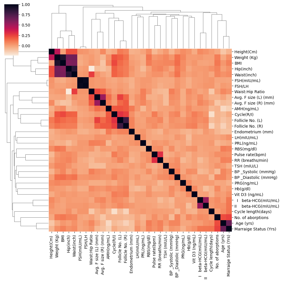
Let’s understand the correlations
sns.clustermap(df_temp.corr(), cmap="rocket_r")
<seaborn.matrix.ClusterGrid at 0x13bf76a50>
df_temp.corr().style.background_gradient(cmap='coolwarm')
| Age (yrs) | Weight (Kg) | Height(Cm) | BMI | Pulse rate(bpm) | RR (breaths/min) | Hb(g/dl) | Cycle(R/I) | Cycle length(days) | Marraige Status (Yrs) | No. of aborptions | I beta-HCG(mIU/mL) | II beta-HCG(mIU/mL) | FSH(mIU/mL) | LH(mIU/mL) | FSH/LH | Hip(inch) | Waist(inch) | Waist:Hip Ratio | TSH (mIU/L) | AMH(ng/mL) | PRL(ng/mL) | Vit D3 (ng/mL) | PRG(ng/mL) | RBS(mg/dl) | BP _Systolic (mmHg) | BP _Diastolic (mmHg) | Follicle No. (L) | Follicle No. (R) | Avg. F size (L) (mm) | Avg. F size (R) (mm) | Endometrium (mm) | |
|---|---|---|---|---|---|---|---|---|---|---|---|---|---|---|---|---|---|---|---|---|---|---|---|---|---|---|---|---|---|---|---|---|
| Age (yrs) | 1.000000 | -0.029136 | -0.118577 | 0.021316 | 0.045553 | 0.086628 | -0.022778 | -0.084871 | 0.055898 | 0.662254 | 0.221843 | 0.008511 | 0.043378 | -0.017708 | 0.000603 | 0.012432 | -0.001346 | 0.036263 | 0.066452 | 0.010245 | -0.179648 | -0.046077 | 0.004454 | -0.021775 | 0.097086 | 0.072313 | 0.069329 | -0.109965 | -0.158865 | -0.017435 | -0.079646 | -0.101969 |
| Weight (Kg) | -0.029136 | 1.000000 | 0.419901 | 0.901755 | 0.020089 | 0.043901 | 0.009979 | 0.200470 | -0.002284 | 0.043991 | 0.093310 | 0.015882 | -0.000521 | -0.025785 | -0.029910 | -0.004831 | 0.633920 | 0.639589 | 0.014976 | 0.071410 | 0.031050 | -0.050016 | 0.008145 | 0.069688 | 0.114294 | 0.028066 | 0.130843 | 0.173501 | 0.124092 | -0.021036 | -0.073115 | -0.010932 |
| Height(Cm) | -0.118577 | 0.419901 | 1.000000 | -0.006906 | -0.074144 | -0.028862 | 0.025259 | -0.018208 | 0.009595 | -0.066407 | -0.026240 | 0.062079 | 0.036474 | 0.030883 | -0.045619 | 0.022065 | 0.215357 | 0.209348 | -0.008982 | 0.018501 | -0.045208 | -0.018178 | -0.034997 | 0.049654 | 0.050437 | -0.067029 | 0.009420 | 0.105574 | 0.074896 | -0.025959 | 0.059686 | -0.055987 |
| BMI | 0.021316 | 0.901755 | -0.006906 | 1.000000 | 0.050536 | 0.061932 | 0.003534 | 0.232891 | -0.006231 | 0.084015 | 0.109865 | -0.009967 | -0.015270 | -0.040717 | -0.013312 | -0.012076 | 0.597058 | 0.607524 | 0.023602 | 0.072305 | 0.054023 | -0.047721 | 0.027035 | 0.049460 | 0.093543 | 0.069549 | 0.140134 | 0.142903 | 0.104205 | -0.011594 | -0.111519 | 0.009320 |
| Pulse rate(bpm) | 0.045553 | 0.020089 | -0.074144 | 0.050536 | 1.000000 | 0.303727 | -0.052265 | 0.101241 | 0.006411 | 0.038701 | 0.046227 | -0.020437 | -0.016226 | -0.013071 | -0.032315 | -0.013104 | 0.062951 | 0.037880 | -0.052890 | -0.051482 | -0.049843 | 0.020750 | -0.001486 | -0.017678 | 0.042002 | -0.025751 | 0.008027 | 0.040559 | 0.049307 | -0.048546 | -0.034256 | -0.040891 |
| RR (breaths/min) | 0.086628 | 0.043901 | -0.028862 | 0.061932 | 0.303727 | 1.000000 | -0.041027 | 0.018850 | 0.004972 | 0.077701 | -0.006090 | -0.085028 | -0.039017 | -0.032388 | -0.031211 | -0.043339 | 0.075020 | 0.038310 | -0.075567 | -0.011968 | -0.017480 | 0.007284 | -0.009016 | -0.076895 | 0.050811 | 0.016734 | 0.053751 | 0.070179 | 0.012752 | -0.031527 | -0.022035 | -0.062941 |
| Hb(g/dl) | -0.022778 | 0.009979 | 0.025259 | 0.003534 | -0.052265 | -0.041027 | 1.000000 | 0.037428 | -0.051992 | 0.006743 | 0.060702 | -0.016649 | -0.094425 | -0.047398 | -0.089107 | -0.039827 | -0.024712 | -0.000779 | 0.057161 | -0.026156 | 0.056172 | -0.063091 | 0.063916 | 0.065769 | 0.024067 | 0.052229 | 0.002046 | 0.061814 | 0.073422 | 0.031995 | 0.024153 | -0.065041 |
| Cycle(R/I) | -0.084871 | 0.200470 | -0.018208 | 0.232891 | 0.101241 | 0.018850 | 0.037428 | 1.000000 | -0.201044 | -0.033557 | -0.057937 | 0.063098 | 0.027930 | -0.026083 | -0.021393 | -0.016167 | 0.174305 | 0.168856 | -0.004003 | -0.017435 | 0.194063 | 0.005251 | 0.096717 | -0.033781 | -0.006394 | 0.055790 | 0.080057 | 0.296114 | 0.251271 | 0.034112 | 0.016204 | 0.042168 |
| Cycle length(days) | 0.055898 | -0.002284 | 0.009595 | -0.006231 | 0.006411 | 0.004972 | -0.051992 | -0.201044 | 1.000000 | 0.117850 | 0.004023 | 0.020187 | 0.018577 | 0.029645 | -0.001686 | 0.025937 | 0.040354 | -0.023479 | -0.130093 | -0.003191 | -0.072822 | 0.016415 | -0.058345 | 0.007190 | 0.000210 | -0.011963 | -0.075792 | -0.086809 | -0.161256 | -0.052364 | -0.013956 | -0.016506 |
| Marraige Status (Yrs) | 0.662254 | 0.043991 | -0.066407 | 0.084015 | 0.038701 | 0.077701 | 0.006743 | -0.033557 | 0.117850 | 1.000000 | 0.246713 | 0.111666 | 0.112905 | -0.023461 | 0.035509 | -0.002983 | 0.038325 | 0.057376 | 0.033334 | -0.040241 | -0.146482 | -0.025819 | 0.041541 | -0.052840 | 0.075519 | 0.028478 | 0.005745 | -0.079079 | -0.087227 | -0.072229 | -0.097536 | -0.105882 |
| No. of aborptions | 0.221843 | 0.093310 | -0.026240 | 0.109865 | 0.046227 | -0.006090 | 0.060702 | -0.057937 | 0.004023 | 0.246713 | 1.000000 | 0.057762 | 0.046977 | -0.018187 | -0.018876 | -0.026472 | 0.078418 | 0.073280 | -0.004031 | 0.032359 | -0.052920 | -0.064655 | 0.015516 | -0.023962 | -0.013134 | -0.083221 | 0.070745 | -0.058061 | -0.078688 | -0.056589 | -0.117573 | -0.067758 |
| I beta-HCG(mIU/mL) | 0.008511 | 0.015882 | 0.062079 | -0.009967 | -0.020437 | -0.085028 | -0.016649 | 0.063098 | 0.020187 | 0.111666 | 0.057762 | 1.000000 | 0.533687 | 0.001641 | -0.006914 | 0.007892 | 0.014833 | 0.005173 | -0.021490 | -0.044710 | 0.014428 | -0.013383 | -0.012659 | -0.002984 | -0.023509 | -0.081720 | 0.003923 | 0.048325 | 0.018266 | 0.050100 | 0.071863 | -0.051920 |
| II beta-HCG(mIU/mL) | 0.043378 | -0.000521 | 0.036474 | -0.015270 | -0.016226 | -0.039017 | -0.094425 | 0.027930 | 0.018577 | 0.112905 | 0.046977 | 0.533687 | 1.000000 | 0.016752 | -0.008092 | 0.027150 | 0.015716 | 0.016541 | 0.001982 | -0.036839 | 0.003668 | -0.001337 | -0.007552 | 0.005649 | -0.004830 | -0.059202 | 0.004021 | 0.064106 | 0.037524 | 0.000003 | 0.037088 | 0.017013 |
| FSH(mIU/mL) | -0.017708 | -0.025785 | 0.030883 | -0.040717 | -0.013071 | -0.032388 | -0.047398 | -0.026083 | 0.029645 | -0.023461 | -0.018187 | 0.001641 | 0.016752 | 1.000000 | -0.001450 | 0.971951 | -0.000158 | 0.013754 | 0.027308 | -0.024805 | -0.014568 | 0.017848 | -0.000683 | -0.003426 | 0.018798 | -0.026830 | 0.023285 | -0.002342 | -0.025358 | 0.011547 | 0.020184 | -0.049158 |
| LH(mIU/mL) | 0.000603 | -0.029910 | -0.045619 | -0.013312 | -0.032315 | -0.031211 | -0.089107 | -0.021393 | -0.001686 | 0.035509 | -0.018876 | -0.006914 | -0.008092 | -0.001450 | 1.000000 | -0.005724 | -0.021727 | -0.022304 | -0.002980 | -0.009398 | 0.021055 | 0.046904 | -0.001543 | -0.004080 | -0.015216 | -0.027699 | 0.023964 | -0.001280 | 0.003430 | 0.035632 | 0.032495 | 0.010786 |
| FSH/LH | 0.012432 | -0.004831 | 0.022065 | -0.012076 | -0.013104 | -0.043339 | -0.039827 | -0.016167 | 0.025937 | -0.002983 | -0.026472 | 0.007892 | 0.027150 | 0.971951 | -0.005724 | 1.000000 | 0.012370 | 0.027588 | 0.029240 | -0.028331 | -0.007438 | 0.015264 | -0.001750 | -0.005109 | 0.006231 | -0.019302 | 0.026920 | 0.005872 | -0.007506 | 0.014923 | 0.024070 | -0.053768 |
| Hip(inch) | -0.001346 | 0.633920 | 0.215357 | 0.597058 | 0.062951 | 0.075020 | -0.024712 | 0.174305 | 0.040354 | 0.038325 | 0.078418 | 0.014833 | 0.015716 | -0.000158 | -0.021727 | 0.012370 | 1.000000 | 0.873589 | -0.241990 | 0.035835 | -0.066106 | -0.082153 | 0.009742 | 0.050008 | -0.001393 | -0.012106 | 0.104944 | 0.119505 | 0.094799 | -0.082276 | -0.104384 | 0.027778 |
| Waist(inch) | 0.036263 | 0.639589 | 0.209348 | 0.607524 | 0.037880 | 0.038310 | -0.000779 | 0.168856 | -0.023479 | 0.057376 | 0.073280 | 0.005173 | 0.016541 | 0.013754 | -0.022304 | 0.027588 | 0.873589 | 1.000000 | 0.258365 | -0.008295 | -0.043132 | -0.036364 | 0.018989 | 0.029175 | 0.012995 | 0.034558 | 0.125243 | 0.129846 | 0.093401 | 0.031048 | -0.015271 | 0.012810 |
| Waist:Hip Ratio | 0.066452 | 0.014976 | -0.008982 | 0.023602 | -0.052890 | -0.075567 | 0.057161 | -0.004003 | -0.130093 | 0.033334 | -0.004031 | -0.021490 | 0.001982 | 0.027308 | -0.002980 | 0.029240 | -0.241990 | 0.258365 | 1.000000 | -0.085023 | 0.057354 | 0.092356 | 0.017701 | -0.039042 | 0.023170 | 0.088978 | 0.042507 | 0.026456 | -0.002207 | 0.229355 | 0.176453 | -0.026793 |
| TSH (mIU/L) | 0.010245 | 0.071410 | 0.018501 | 0.072305 | -0.051482 | -0.011968 | -0.026156 | -0.017435 | -0.003191 | -0.040241 | 0.032359 | -0.044710 | -0.036839 | -0.024805 | -0.009398 | -0.028331 | 0.035835 | -0.008295 | -0.085023 | 1.000000 | -0.010854 | 0.025606 | -0.009114 | -0.020504 | -0.030056 | 0.048215 | 0.055034 | -0.028164 | -0.016807 | -0.091201 | -0.088850 | 0.013863 |
| AMH(ng/mL) | -0.179648 | 0.031050 | -0.045208 | 0.054023 | -0.049843 | -0.017480 | 0.056172 | 0.194063 | -0.072822 | -0.146482 | -0.052920 | 0.014428 | 0.003668 | -0.014568 | 0.021055 | -0.007438 | -0.066106 | -0.043132 | 0.057354 | -0.010854 | 1.000000 | -0.072214 | 0.007660 | -0.011195 | 0.008454 | -0.003192 | 0.026038 | 0.203407 | 0.188537 | 0.134628 | 0.096079 | 0.104159 |
| PRL(ng/mL) | -0.046077 | -0.050016 | -0.018178 | -0.047721 | 0.020750 | 0.007284 | -0.063091 | 0.005251 | 0.016415 | -0.025819 | -0.064655 | -0.013383 | -0.001337 | 0.017848 | 0.046904 | 0.015264 | -0.082153 | -0.036364 | 0.092356 | 0.025606 | -0.072214 | 1.000000 | -0.006827 | -0.009700 | -0.041676 | -0.009963 | -0.026821 | -0.010803 | -0.008607 | 0.086311 | 0.071688 | 0.027439 |
| Vit D3 (ng/mL) | 0.004454 | 0.008145 | -0.034997 | 0.027035 | -0.001486 | -0.009016 | 0.063916 | 0.096717 | -0.058345 | 0.041541 | 0.015516 | -0.012659 | -0.007552 | -0.000683 | -0.001543 | -0.001750 | 0.009742 | 0.018989 | 0.017701 | -0.009114 | 0.007660 | -0.006827 | 1.000000 | -0.007240 | 0.038980 | 0.042855 | -0.024962 | 0.074172 | 0.091775 | 0.005441 | -0.011812 | -0.031385 |
| PRG(ng/mL) | -0.021775 | 0.069688 | 0.049654 | 0.049460 | -0.017678 | -0.076895 | 0.065769 | -0.033781 | 0.007190 | -0.052840 | -0.023962 | -0.002984 | 0.005649 | -0.003426 | -0.004080 | -0.005109 | 0.050008 | 0.029175 | -0.039042 | -0.020504 | -0.011195 | -0.009700 | -0.007240 | 1.000000 | -0.003545 | -0.020638 | 0.032131 | 0.018489 | 0.031483 | -0.040698 | -0.040910 | -0.047987 |
| RBS(mg/dl) | 0.097086 | 0.114294 | 0.050437 | 0.093543 | 0.042002 | 0.050811 | 0.024067 | -0.006394 | 0.000210 | 0.075519 | -0.013134 | -0.023509 | -0.004830 | 0.018798 | -0.015216 | 0.006231 | -0.001393 | 0.012995 | 0.023170 | -0.030056 | 0.008454 | -0.041676 | 0.038980 | -0.003545 | 1.000000 | 0.052683 | -0.032907 | 0.044342 | 0.027562 | -0.046821 | 0.013137 | -0.018700 |
| BP _Systolic (mmHg) | 0.072313 | 0.028066 | -0.067029 | 0.069549 | -0.025751 | 0.016734 | 0.052229 | 0.055790 | -0.011963 | 0.028478 | -0.083221 | -0.081720 | -0.059202 | -0.026830 | -0.027699 | -0.019302 | -0.012106 | 0.034558 | 0.088978 | 0.048215 | -0.003192 | -0.009963 | 0.042855 | -0.020638 | 0.052683 | 1.000000 | 0.102090 | 0.039463 | 0.025515 | 0.051273 | 0.038448 | -0.018613 |
| BP _Diastolic (mmHg) | 0.069329 | 0.130843 | 0.009420 | 0.140134 | 0.008027 | 0.053751 | 0.002046 | 0.080057 | -0.075792 | 0.005745 | 0.070745 | 0.003923 | 0.004021 | 0.023285 | 0.023964 | 0.026920 | 0.104944 | 0.125243 | 0.042507 | 0.055034 | 0.026038 | -0.026821 | -0.024962 | 0.032131 | -0.032907 | 0.102090 | 1.000000 | 0.025043 | 0.037844 | 0.037028 | 0.024013 | -0.015342 |
| Follicle No. (L) | -0.109965 | 0.173501 | 0.105574 | 0.142903 | 0.040559 | 0.070179 | 0.061814 | 0.296114 | -0.086809 | -0.079079 | -0.058061 | 0.048325 | 0.064106 | -0.002342 | -0.001280 | 0.005872 | 0.119505 | 0.129846 | 0.026456 | -0.028164 | 0.203407 | -0.010803 | 0.074172 | 0.018489 | 0.044342 | 0.039463 | 0.025043 | 1.000000 | 0.799516 | 0.249781 | 0.149002 | 0.078605 |
| Follicle No. (R) | -0.158865 | 0.124092 | 0.074896 | 0.104205 | 0.049307 | 0.012752 | 0.073422 | 0.251271 | -0.161256 | -0.087227 | -0.078688 | 0.018266 | 0.037524 | -0.025358 | 0.003430 | -0.007506 | 0.094799 | 0.093401 | -0.002207 | -0.016807 | 0.188537 | -0.008607 | 0.091775 | 0.031483 | 0.027562 | 0.025515 | 0.037844 | 0.799516 | 1.000000 | 0.156640 | 0.188049 | 0.079817 |
| Avg. F size (L) (mm) | -0.017435 | -0.021036 | -0.025959 | -0.011594 | -0.048546 | -0.031527 | 0.031995 | 0.034112 | -0.052364 | -0.072229 | -0.056589 | 0.050100 | 0.000003 | 0.011547 | 0.035632 | 0.014923 | -0.082276 | 0.031048 | 0.229355 | -0.091201 | 0.134628 | 0.086311 | 0.005441 | -0.040698 | -0.046821 | 0.051273 | 0.037028 | 0.249781 | 0.156640 | 1.000000 | 0.522794 | -0.014174 |
| Avg. F size (R) (mm) | -0.079646 | -0.073115 | 0.059686 | -0.111519 | -0.034256 | -0.022035 | 0.024153 | 0.016204 | -0.013956 | -0.097536 | -0.117573 | 0.071863 | 0.037088 | 0.020184 | 0.032495 | 0.024070 | -0.104384 | -0.015271 | 0.176453 | -0.088850 | 0.096079 | 0.071688 | -0.011812 | -0.040910 | 0.013137 | 0.038448 | 0.024013 | 0.149002 | 0.188049 | 0.522794 | 1.000000 | -0.045628 |
| Endometrium (mm) | -0.101969 | -0.010932 | -0.055987 | 0.009320 | -0.040891 | -0.062941 | -0.065041 | 0.042168 | -0.016506 | -0.105882 | -0.067758 | -0.051920 | 0.017013 | -0.049158 | 0.010786 | -0.053768 | 0.027778 | 0.012810 | -0.026793 | 0.013863 | 0.104159 | 0.027439 | -0.031385 | -0.047987 | -0.018700 | -0.018613 | -0.015342 | 0.078605 | 0.079817 | -0.014174 | -0.045628 | 1.000000 |
Correlation analysis
So far we did nott split the data on PCOS diagnosis. Our next task is to do that. Let’s make to different dataframes:
- contains PCOS diagnosis
- does not contain PCOS diagnosis
This should not be strictly necessary, but I am just playing around pandas here.
df_PCOS = df_PCOS_all[df_PCOS_all['PCOS (Y/N)']]
df_no_PCOS = df_PCOS_all[~df_PCOS_all['PCOS (Y/N)']]
df_no_PCOS
| Sl. No | Patient File No. | PCOS (Y/N) | Age (yrs) | Weight (Kg) | Height(Cm) | BMI | Blood Group | Pulse rate(bpm) | RR (breaths/min) | ... | Fast food (Y/N) | Reg.Exercise(Y/N) | BP _Systolic (mmHg) | BP _Diastolic (mmHg) | Follicle No. (L) | Follicle No. (R) | Avg. F size (L) (mm) | Avg. F size (R) (mm) | Endometrium (mm) | Unnamed: 44 | |
|---|---|---|---|---|---|---|---|---|---|---|---|---|---|---|---|---|---|---|---|---|---|
| 0 | 1 | 1 | False | 28 | 44.6 | 152.000 | 19.300000 | 15 | 78 | 22 | ... | True | False | 110 | 80 | 3 | 3 | 18.0 | 18.0 | 8.5 | NaN |
| 1 | 2 | 2 | False | 36 | 65.0 | 161.500 | 24.921163 | 15 | 74 | 20 | ... | False | False | 120 | 70 | 3 | 5 | 15.0 | 14.0 | 3.7 | NaN |
| 3 | 4 | 4 | False | 37 | 65.0 | 148.000 | 29.674945 | 13 | 72 | 20 | ... | False | False | 120 | 70 | 2 | 2 | 15.0 | 14.0 | 7.5 | NaN |
| 4 | 5 | 5 | False | 25 | 52.0 | 161.000 | 20.060954 | 11 | 72 | 18 | ... | False | False | 120 | 80 | 3 | 4 | 16.0 | 14.0 | 7.0 | NaN |
| 5 | 6 | 6 | False | 36 | 74.1 | 165.000 | 27.217631 | 15 | 78 | 28 | ... | False | False | 110 | 70 | 9 | 6 | 16.0 | 20.0 | 8.0 | NaN |
| ... | ... | ... | ... | ... | ... | ... | ... | ... | ... | ... | ... | ... | ... | ... | ... | ... | ... | ... | ... | ... | ... |
| 535 | 536 | 536 | False | 26 | 80.0 | 161.544 | 30.700000 | 18 | 70 | 18 | ... | False | False | 110 | 80 | 7 | 9 | 13.0 | 17.5 | 9.6 | NaN |
| 536 | 537 | 537 | False | 35 | 50.0 | 164.592 | 18.500000 | 17 | 72 | 16 | ... | False | False | 110 | 70 | 1 | 0 | 17.5 | 10.0 | 6.7 | NaN |
| 537 | 538 | 538 | False | 30 | 63.2 | 158.000 | 25.300000 | 15 | 72 | 18 | ... | False | False | 110 | 70 | 9 | 7 | 19.0 | 18.0 | 8.2 | NaN |
| 538 | 539 | 539 | False | 36 | 54.0 | 152.000 | 23.400000 | 13 | 74 | 20 | ... | False | False | 110 | 80 | 1 | 0 | 18.0 | 9.0 | 7.3 | NaN |
| 539 | 540 | 540 | False | 27 | 50.0 | 150.000 | 22.200000 | 15 | 74 | 20 | ... | False | False | 110 | 70 | 7 | 6 | 18.0 | 16.0 | 11.5 | NaN |
363 rows × 45 columns
# We have to use Perason's correlation coefficient because the dataframe contains both boolean and integer values.
corr = df_PCOS_all.drop(columns_to_drop, axis = 1).corr(method ='pearson')
# Let's try to extract the variables which have the highest and lowest correlation with PCOS status.
print(f' The three highest {list(corr.nlargest(3, "PCOS (Y/N)")["PCOS (Y/N)"].index)}')
print(f' The three smallest PCOS correlated variables are {list(corr.nsmallest(3, "PCOS (Y/N)")["PCOS (Y/N)"].index)}')
 The three highest ['PCOS (Y/N)', 'Follicle No. (R)', 'Follicle No. (L)']
 The three smallest PCOS correlated variables are ['Cycle length(days)', ' Age (yrs)', 'Marraige Status (Yrs)']
Checking the positive and negative correlations seperately
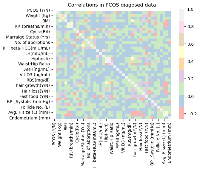
Do the correlation matrices of PCOS diagnosis vs no PCOS diagnosis look very different?
corrpos = df_PCOS.drop(columns_to_drop, axis = 1).corr()
corrneg = df_no_PCOS.drop(columns_to_drop, axis = 1).corr()
sns.heatmap(corrpos, cmap="Pastel1")
plt.title('Correlations in PCOS diagosed data');
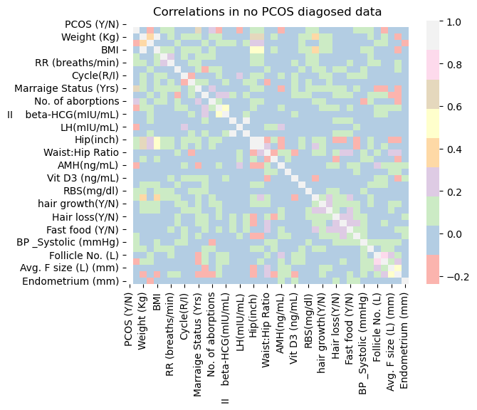
sns.heatmap(corrneg, cmap="Pastel1")
plt.title('Correlations in no PCOS diagosed data');
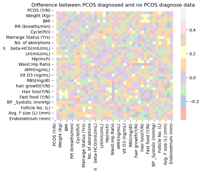
sns.heatmap(corrpos-corrneg, cmap="Pastel1")
plt.title('Difference between PCOS diagnosed and no PCOS diagnose data');
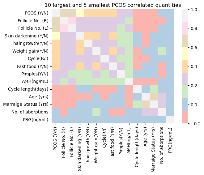
For simplicity I would want to plot the 10 highest PCOS correlated and 5 lowest correlated variables as a heatmap.
#print(df_PCOS_all.describe())
#columns_to_drop = ['Sl. No', 'Patient File No.', 'Blood Group']
largest_vars = corr.nlargest(10, "PCOS (Y/N)")["PCOS (Y/N)"].index
smallest_vars = corr.nsmallest(5, "PCOS (Y/N)")["PCOS (Y/N)"].index
total_vars = largest_vars.append(smallest_vars)
sns.heatmap(df_PCOS_all.drop(columns_to_drop, axis=1)[total_vars].corr(), \
            cmap = "Pastel1")
plt.title('10 largest and 5 smallest PCOS correlated quantities');
Visualise PCOS true and PCOS false data distributions
df_PCOS_numeric = df_PCOS.select_dtypes(exclude = 'bool')
df_PCOS_numeric = df_PCOS_numeric.drop(columns_to_drop, axis = 1)
df_no_PCOS_numeric = df_no_PCOS.select_dtypes(exclude = 'bool')
df_no_PCOS_numeric = df_no_PCOS_numeric.drop(columns_to_drop, axis = 1)
variable_dropdown = Dropdown(options = df_PCOS_numeric.columns)
output_plot = Output()

def make_histograms(*args):
    output_plot.clear_output(wait = True)
    with output_plot:
        fig, ax1 = plt.subplots()
        sns.histplot(x = variable_dropdown.value, data = df_PCOS, kde = True, ax = ax1 )
        sns.histplot(x = variable_dropdown.value, data = df_no_PCOS, kde = True, ax = ax1)
        #ax1.get_legend()
        #legend = ax1.get_legend()
        #handles = legend.legend_handles
        #ax1.legend(handles, ['PCOS True', 'PCOS False'], title='Stat.ind.')
        plt.show()

variable_dropdown.observe(make_histograms, names = 'value')
display(variable_dropdown, output_plot)
Dropdown(options=(' Age (yrs)', 'Weight (Kg)', 'Height(Cm) ', 'BMI', 'Pulse rate(bpm) ', 'RR (breaths/min)', '…


Output()
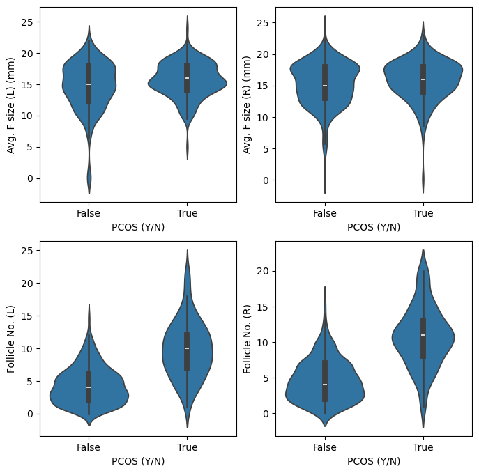
Among all the plots we can look at above the plots related to left and right follicle measurements are distinctly different. Let’s look at them in a bit more detail.
fig, ax = plt.subplots(2,2, figsize = (8,8))
sns.violinplot(df_PCOS_all, x = 'PCOS (Y/N)', y = 'Avg. F size (L) (mm)', ax = ax[0][0])
sns.violinplot(df_PCOS_all, x = 'PCOS (Y/N)', y = 'Avg. F size (R) (mm)', ax = ax[0][1])
sns.violinplot(df_PCOS_all, x = 'PCOS (Y/N)', y = 'Follicle No. (L)', ax = ax[1][0])
sns.violinplot(df_PCOS_all, x = 'PCOS (Y/N)', y = 'Follicle No. (R)', ax = ax[1][1])
<Axes: xlabel='PCOS (Y/N)', ylabel='Follicle No. (R)'>
Statistical analysis
My main goal is to be able to understand which factors are correlated with PCOS. These are not ‘causes’ of PCOS but rather symtoms which can help diagnose the condition. Note that correlations within binary data are also computed in .corr() method of pandas. Here I evaluate them explicitly.
Evaluating Cramér’s V coefficient
Cramér’s V coefficient is used for evaluating correlation between two variables. The variables may have more than binary categories. For variables A, B if
$n_{i,j}$ = number of times $A_i, B_j$ were observed,
$\chi^2 = \sum_{i,j}\frac{(n_{i,j} - {\frac{n_i, n_j}{n}})}{\frac{n_i, n_j}{n}}$
where $n_i = \sum_j n_{i,j}$ is the number of times the value $A_i$ is observed and $n_i = \sum_j n_{i,j}$ is the number of times the value $B_j$ is observed.
The coefficient is the computed as
$V = \sqrt\frac{\chi^2/n}{min(k-1)(r-1)}$
where $k$ = number of columns, $r$ = number of rows, $n$ = total number of observations
from scipy.stats import chi2_contingency
from tabulate import tabulate
import numpy as np
df_PCOS_bool = df_PCOS_all.select_dtypes(include = 'bool')
results = []
for col in df_PCOS_bool.columns:
    if col == 'PCOS (Y/N)': continue
    pearson_corr = df_PCOS_bool['PCOS (Y/N)'].astype(int).corr(df_PCOS_bool[col].astype(int))
    # Now let's compute the Cramér's V coefficient
    contigency_table = pd.crosstab(df_PCOS_bool['PCOS (Y/N)'].astype(int), df_PCOS_bool[col].astype(int))
    print('----------------------------------')
    print(contigency_table )

    chi2, _, _, _ = chi2_contingency(contigency_table)
    n = contigency_table.values.sum()
    cramers_v = np.sqrt(chi2/n)
    results.append([col, pearson_corr, cramers_v])
print('----------------------------------')
print(tabulate(results, headers = ['criteria', 'Pearsons coefficient', 'cramers_v']))
----------------------------------
Pregnant(Y/N)    0    1
PCOS (Y/N)
0              221  142
1              113   64
----------------------------------
Weight gain(Y/N)    0    1
PCOS (Y/N)
0                 280   83
1                  56  121
----------------------------------
hair growth(Y/N)    0    1
PCOS (Y/N)
0                 316   47
1                  76  101
----------------------------------
Skin darkening (Y/N)    0    1
PCOS (Y/N)
0                     307   56
1                      67  110
----------------------------------
Hair loss(Y/N)    0    1
PCOS (Y/N)
0               220  143
1                75  102
----------------------------------
Pimples(Y/N)    0    1
PCOS (Y/N)
0             222  141
1              54  123
----------------------------------
Fast food (Y/N)    0    1
PCOS (Y/N)
0                223  140
1                 38  139
----------------------------------
Reg.Exercise(Y/N)    0   1
PCOS (Y/N)
0                  281  82
1                  126  51
----------------------------------
criteria                Pearsons coefficient    cramers_v
--------------------  ----------------------  -----------
Pregnant(Y/N)                     -0.0286064    0.0245456
Weight gain(Y/N)                   0.440488     0.436419
hair growth(Y/N)                   0.464245     0.459823
Skin darkening (Y/N)               0.475283     0.471008
Hair loss(Y/N)                     0.171913     0.167951
Pimples(Y/N)                       0.287802     0.283856
Fast food (Y/N)                    0.375389     0.371442
Reg.Exercise(Y/N)                  0.0678092    0.0632309
It seems that hair growth, skin darknin and hair loss are correlated with PCOS diagnosis. Fast food seems to have a correlation but I wonder if that is an artefact.
Training a classifier (Random Forest)
I will use a random forrest classifier here because there is no specific knowledge to choose other classifiers. In addition, the data consists of both integers and boolaen types. I believe that random forest classifier should work.
$precision = \frac{TP}{TP+FP}$
$recall = \frac{TP}{FP+FN}$
$F_1 score = \frac{precision \times recall}{precision + recall}$
from sklearn.model_selection import train_test_split, cross_val_predict
from sklearn.ensemble import RandomForestClassifier
from sklearn.metrics import accuracy_score, classification_report, confusion_matrix, precision_recall_curve
from sklearn.preprocessing import StandardScaler

columns_to_convert = df_PCOS_all.filter(like = 'Y/N').columns
df_PCOS_all[columns_to_convert] = df_PCOS_all[columns_to_convert].astype('int')

label_col = "PCOS (Y/N)"
X = df_PCOS_all.drop(columns = [label_col])
X = X.drop(columns = columns_to_drop, axis = 1)

y = df_PCOS_all[label_col]

float_columns = X.select_dtypes(include = ['float64']).columns

scaler=StandardScaler()
X[float_columns] = scaler.fit_transform(X[float_columns])

X_train, X_test, y_train, y_test = train_test_split(X, y, test_size = 0.2)

clf = RandomForestClassifier()

clf.fit(X_train, y_train)
y_pred = clf.predict(X_test)

accuracy = accuracy_score(y_test, y_pred)
print(f'Accuracy is {accuracy}')

print('\n Classification report is')
print(classification_report(y_test, y_pred))

# Optional: Display the confusion matrix
conf_matrix = confusion_matrix(y_test, y_pred)
print("\n Confusion Matrix:")
print('\n'.join(['\t'.join([str(cell) for cell in row]) for row in conf_matrix]))
Accuracy is 0.8888888888888888

 Classification report is
              precision    recall  f1-score   support

           0       0.87      0.97      0.92        71
           1       0.93      0.73      0.82        37

    accuracy                           0.89       108
   macro avg       0.90      0.85      0.87       108
weighted avg       0.89      0.89      0.89       108


 Confusion Matrix:
69	2
10	27
The above scores don’t look too bad.
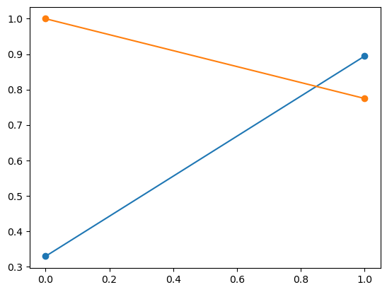
Let us try to make a precisio vs recall curve. The following curve doesn’t look right, so I have to do something to fix it.
y_scores = cross_val_predict(clf, X_train, y_train)#, method = 'decision_function')
precisions, recalls, thresholds = precision_recall_curve(y_train, y_scores)
print(precisions,recalls, thresholds)
plt.plot(thresholds, precisions[:-1])
plt.plot(thresholds, recalls[:-1])
plt.scatter(thresholds, precisions[:-1])
plt.scatter(thresholds, recalls[:-1])
[0.3287037  0.89430894 1.        ] [1.         0.77464789 0.        ] [0 1]


<matplotlib.collections.PathCollection at 0x15f8de990>
Hypothesis testing (next step)
see https://towardsdatascience.com/hypothesis-testing-with-python-step-by-step-hands-on-tutorial-with-practical-examples-e805975ea96e for hypothesis testing